Overview

Generative Adversarial Networks (GANs) are a class of deep learning methods which is first proposed by Ian Goodfellow and other researchers at the University of Montreal in 2014 [1]. Two neural networks, a generator, and a discriminator learn in a zero-sum game framework.

The loss formulation of GAN is as follows:

$$ \min_{G} \ \max_{D}V(D,G)= \mathbb{E}_{x\sim p_{data}(x)}\big[ \log D(x) \big] + \mathbb{E}_{z\sim p_{z}(z)} \big[ \log (1- D(G(z))) \big]$$

By sampling from a uniform distribution, generator tries to capture the data distribution, whereas discriminator estimates whether a data sample comes from the real distribution or G. Generator is learned to maximize the probability of D making a mistake.

Since the first paper, GAN variants have shown promising results; however, they suffer from several problems, too. The balance of generator and discriminator is difficult, and there are many situations where gradients may diminish, or the model oscillate and never converges. Even in the success case, there is no guarantee that the latent space represents each node of the real data distribution (mode collapse). Furthermore, the training of GANs is highly sensitive to hyperparameter selection.

In this blog post, I will briefly summarize the additional tricks which lead to better performance of GANs (by reducing the chance of these problems happen), an example of GAN method which produces high-resolution images and an example of conditional GANs, image-to-image translation.

Improved techniques to train GANs

The network architectures in the original paper were fully connected layers. Radford et al. [2] replaced any pooling layers with strided convolutions and fractional strided convolutions in D and G, removed fully connected hidden layers, used batch normalization. They also used ReLU activations in all layers of G, except for the output which uses tanh. By making these improvements, they achieved a good improvement and showed experimental results in face and scene generation.

Salimans et al. [3] propose several tricks to improve the performance of GAN training. We can shortly summarize them as follows:

• Feature matching: letting $f(x)$ denote activations on an intermediate layer of discriminator (or another pre-trained net)

  • $ || \mathbb{E}_{x\sim p_{data}}\ f(x) - \mathbb{E}_{z\sim p_{z}} \ f(G(z))||_2^2 $

• Minibatch discrimination: (to encourage diversity)

  • Let $f(x_i) \in \mathbb{R}^A$, $T \in \mathbb{R}^{A\times B \times C}$ a tensor, $f(x_i) \times T=M_i \in \mathbb{R}^{B \times C}$
    
  • Compute the $L_1$ distances between rows of $M_i$ and apply a negative exponential: $$c_b(x_i, x_j)= \exp(- ||M_{i,b} - M_{j,b}||_{L_1}) \in \mathbb{R} $$

• Historical Averaging: learning rule scales well in time.

  • (loosely inspired by the fictitious play that can find equilibria) $|| \ \theta - \frac{1}{t}\sum_{i=1}^{t} \theta[i] \ ||^2$

• (One-sided) label smoothing: In the output of D, real images’ outputs smoothed to avoid overconfidence.

• Other practical tricks to stabilize DC-GAN-like networks: https://github.com/soumith/ganhacks

Generating High-Quality Images

In addition to the previously mentioned tricks to improve GAN performance, there were many advances in GAN variants, particularly in their loss formulation. The original GAN’s discriminator is a classifier with a sigmoid cross-entropy loss function (which may lead to vanishing gradient problems), and it was difficult to optimize Jensen-Shannon divergence in case of little or no overlap between two distributions. [4] adopted the least squares loss function for the discriminator. They show that minimizing the Pearson $\chi^2$ divergence. Another work [5,6] used Wasserstein 1 (Earth-Movers) loss function which has a smooth differentiable function almost everywhere.

Let us look at an example of GAN algorithm which yields photorealistic, high-resolution images: Progressive growing of GANs [7]. The key idea is “to grow both the generator and discriminator progressively: starting from a low resolution, we add new layers that model increasingly fine details as training progresses. This both speeds the training up and greatly stabilizes it, allowing to produce images of unprecedented quality.”

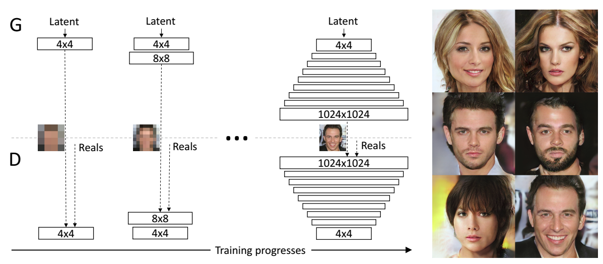
Progressive GANs’ main loss is based on improved Wasserstein GAN [6]. As well as progressive growth idea, there are other important points which lead to the diversity and photorealism of their generated images:

• Minibatch stddev: adding the across.minibatch standard deviation as an additional feature map.

• Equalized learning rate: initializing weights trivially by normal dist. with unit variance and normalize by a constant layerwise coefficient (He et al. 2015), $\hat{w}_i=w_i/c$

• Pixelwise feature normalization in G

  • $b_{x,y}=a_{x,y} / \sqrt{\frac{1}{N} \sum_{j=0}^{N-1} (a_{x,y}^j)^2+\epsilon}$

A follow-up work from the authors of Progressive-GAN, Style-GAN [8]. Their main contribution is to integrate generator network the ability to control different levels of features (“styles”). “Generator starts from a learned constant input and adjusts the style of the image at each convolution layer based on the latent code, therefore directly controlling the strength of image features at different scales.”

They defined three levels of styles as follows:

• coarse ($4^2 -8^2$) pose, general hairstyle, face shape
• middle ($16^2-32^2$) facial features, hairstyle, eyes open/closed
• fine ($64^2 - 1024^2$) color scheme (eye, hair, and skin) and micro features.

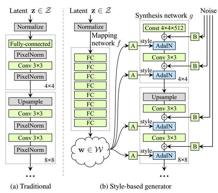
In the training procedure of generator, the input vector is encoded by a mapping network first before fed into the generator. In this way, they control different visual features. In each resolution, a learned affine transformation applied into the output of mapping network,$W$ and they are converted to “style” representations. Then, an instant normalization (AdaIN) which is adapted by style $y$.
$$AdaIN(x_i,y)= y_{s,i}\frac{x_i - \mu(x_i)}{\sigma(x_i)} + y_{b,i}$$
The adaptive instance normalization and adding style in different resolutions give the chance to disentangle the latent space in varying granularities. In addition to the attributed which can be disentangled, they add noise in different levels to have additional variations (for instance, freckles).

One of the important problems of GANs is the poorly represented areas where the generator has difficulty to learn. Thus, they apply a truncation in following way: After some training, first compute the center of mass of $\mathcal{W}$ as $\hat{w}=\mathbb{E}_{z\sim P(z)} [f(z)]$ and scale the deviation of a given $w$ from the center as $\hat{w}=\hat{w}+\psi(w-\hat{w})$ where $\psi \le 1$.

Image-to-Image Translation

In the original GAN idea and the examples covered in the previous section, generators learn the distribution only from the uniform of Gaussian distributions. A line of work, conditional GANs learn the distribution from the noise and some structural information such as a label, attribute or a feature representation. We can compare the loss formulation of unconditional and conditional GAN as follows:

• $G:z\rightarrow y$

  • Standard GAN’s learn a mapping from random noise $z$ to output image $y$
  • $\mathcal{L}_{GAN}(G,D)=\mathbb{E} [ \log D(y)] + \mathbb{E}_{x,z} [ \log (1-D(G(x,z))) ]$

• $G:{x,z}\rightarrow y$

  • Conditional GAN’s learn a mapping from observed data $x$ and random noise $z$ to output image.
  • $\mathcal{L}_{cGAN}(G,D)=\mathbb{E} [ \log D(x,y)] + \mathbb{E}_{x,z} [ \log (1-D(x, G(x,z))) ]$

• Adding an L2 or (the better one) L1 regularization in G.

  • $\mathcal{L}_{L1}(G)=\mathbb{E}_{x,y,z}[ \ || y-G(x,z) ||_1 \ ]$
  • $\mathcal{L}_{cGAN}(G,D) + \mathcal{L}_{L1}(G)$

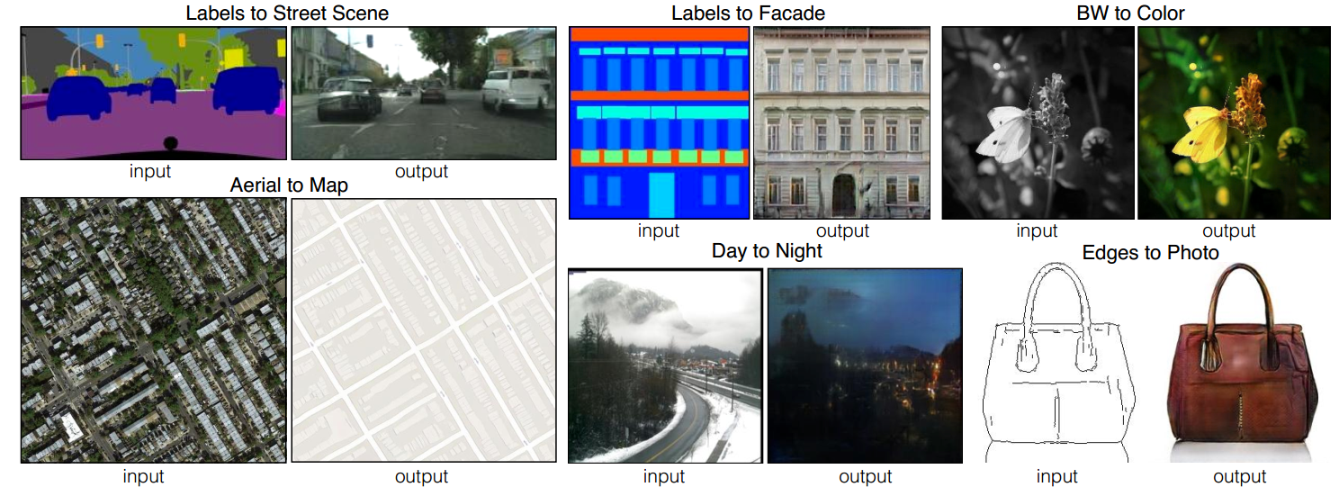
By adding an $L_1$ regression to conditional GAN, Isola et al. ($\texttt{pix2pix}$) [9] proposed a mapping between paired image domains such as aerial images$\leftrightarrow$maps, image$\leftrightarrow$painting, winter$\leftrightarrow$summer, and so on.

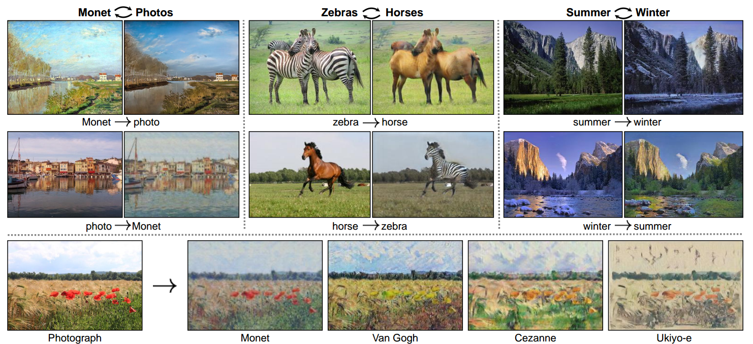
Their results were quite impressive, but it is not easy to find paired dataset (automatically without manual labeling cost). The same authors in a follow-up work ($\texttt{CycleGAN}$) [10] showed that translations could be done even between unpaired domains. In CycleGAN, there are two discriminators and generators.

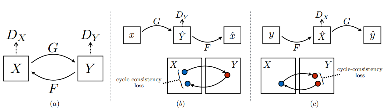
In addition to adversarial losses, they minimize two $L_1$ terms between the original domain and its remapped version in both sides.

$$\mathcal{L}_{GAN}(G,D_Y,X,Y)=\mathbb{E}_{y\sim p_{data}(y)} [ \log D_Y(y)] + \mathbb{E}_{x \sim p_{data}(x)} [ \log (1-D_Y(G(x))) ]$$

$$\mathcal{L}_{cyc}(G,F)=\mathbb{E}_{x \sim p_{data}(x)}[ \ ||F(G(x))-x||_1 ] + \mathbb{E}_{y\sim p_{data}(y)}[ \ ||G(F(y))-y||_1 ]$$

And full objective function is
$$\mathcal{L}(G,F,D_X,D_Y)=\mathcal{L}_{GAN}(G,D_Y,X,Y)+\mathscr{L}_{GAN}(F,D_X,Y,X)+\lambda \mathscr{L}_{cyc}(G,F)$$

Here are some examples of CycleGAN:

There are many recent works which aim to disentangle feature representations in latent space. Most of them depend on the idea of pix2pix or CycleGAN. For instance, generating images or videos by conditioned on two different images’ pose and appearance and combine them, face swapping, style transfer, etc. Here are two examples:

• Liqian Ma, Qianru Sun, Stamatios Georgoulis, Luc Van Gool, Bernt Schiele, Mario Fritz, “Disentangled Person Image Generation,” The IEEE Conference on Computer Vision and Pattern Recognition (CVPR), 2018, (video)

• Caroline Chan, Shiry Ginosar, Tinghui Zhou, Alexei A. Efros, “Everybody Dance Now,” 2018, http://arxiv.org/abs/1808.07371, (video).

Conclusion

In this blog post, I briefly described the additional tricks which make the original GAN idea to fully equipped to generate high-resolution images and image-to-image translation as an example of conditioned GANs.

There are many qualitative and quantitative measures to compare generated images, and it is always possible to go further generating more realistic data samples. However, from my point of view, these are the points which make them (and other generative models) interesting:

• The power of unsupervised representation by showing the performance of D’s features in image retrieval, classification tasks.
• Adding adversarial term to supervised learning to make them perform better, for instance, pose estimation, facial keypoint detection, person identification, etc.)
• Augmenting the data especially less sampled nodes.
• Towards more structural latent encoding. The recent works try to disentangle into interpretable features in an unsupervised manner.

References

[1] Ian J. Goodfellow, Jean Pouget-Abadie, Mehdi Mirza, Bing Xu, David Warde-Farley, Sherjil Ozair, Aaron Courville, and Yoshua Bengio, “Generative adversarial nets,” International Conference on Neural Information Processing Systems (NeurIPS), 2014.

[2] Alec Radford, Luke Metz, and Soumith Chintala, Unsupervised Representation Learning with Deep Convolutional Generative Adversarial Networks, International Conference on Learning Representations (ICLR), 2016.

[3] Tim Salimans, Ian Goodfellow, Wojciech Zaremba, Vicki Cheung, Alec Radford, and Xi Chen. 2016. Improved techniques for training GANs,” International Conference on Neural Information Processing Systems (NeurIPS), 2016.

[4] Xudong Mao, Li Qing, Xie Haoran, Y. K. Lau Raymond, Wang Zhen, and Stephen Paul Smolley, “Least Squares Generative Adversarial Networks.” IEEE International Conference on Computer Vision (ICCV), 2017.

[5] Martin Arjovsky, Soumith Chintala, Léon Bottou, “Wasserstein Generative Adversarial Networks,” Proceedings of the 34th International Conference on Machine Learning, PMLR 70:214-223, 2017.

[6] Ishaan Gulrajani, Faruk Ahmed, Martin Arjovsky, Vincent Dumoulin, and Aaron Courville, “Improved Training of Wasserstein GANs,” International Conference on Neural Information Processing Systems (NeurIPS), 2016.

[7] Tero Karras, Timo Aila, Samuli Laine, and Jaakko Lehtinen. “Progressive Growing of GANs for Improved Quality, Stability, and Variation,” International Conference on Learning Representations (ICLR), 2018.

[8] Tero Karras, Samuli Laine, Timo Aila, “A Style-Based Generator Architecture for Generative Adversarial Networks,” https://arxiv.org/abs/1812.04948

[9] Phillip Isola, Jun-Yan Zhu, Tinghui Zhou, and Alexei A. Efros, “Image-to-Image Translation with Conditional Adversarial Networks,” 2017 IEEE Conference on Computer Vision and Pattern Recognition (CVPR), 2017.

[10] Jun-Yan Zhu, Taesung Park, Phillip Isola, and Alexei A. Efros, “Unpaired Image-to-Image Translation Using Cycle-Consistent Adversarial Networks,” 2017 IEEE International Conference on Computer Vision (ICCV), 2017.